- 您現(xiàn)在的位置:買(mǎi)賣(mài)IC網(wǎng) > PDF目錄373942 > AD8307 (Analog Devices, Inc.) Low Cost DC-500 MHz, 92 dB Logarithmic Amplifier(對(duì)數(shù)放大器) PDF資料下載
參數(shù)資料
| 型號(hào): | AD8307 |
| 廠商: | Analog Devices, Inc. |
| 元件分類(lèi): | 運(yùn)動(dòng)控制電子 |
| 英文描述: | Low Cost DC-500 MHz, 92 dB Logarithmic Amplifier(對(duì)數(shù)放大器) |
| 中文描述: | 低成本DC - 500兆赫,九十二分貝對(duì)數(shù)放大器(對(duì)數(shù)放大器) |
| 文件頁(yè)數(shù): | 8/20頁(yè) |
| 文件大小: | 303K |
| 代理商: | AD8307 |
第1頁(yè)第2頁(yè)第3頁(yè)第4頁(yè)第5頁(yè)第6頁(yè)第7頁(yè)當(dāng)前第8頁(yè)第9頁(yè)第10頁(yè)第11頁(yè)第12頁(yè)第13頁(yè)第14頁(yè)第15頁(yè)第16頁(yè)第17頁(yè)第18頁(yè)第19頁(yè)第20頁(yè)
AD8307
–8–
REV. 0
voltage. T he use of dBV (decibels with respect to 1 V rms) would
be more precise, though still incomplete, since waveform is
involved, too. Since most users think about and specify
RF
signals in terms of power—even more specifically, in dBm re 50
—we will use this convention in specifying the performance of
the AD8307.
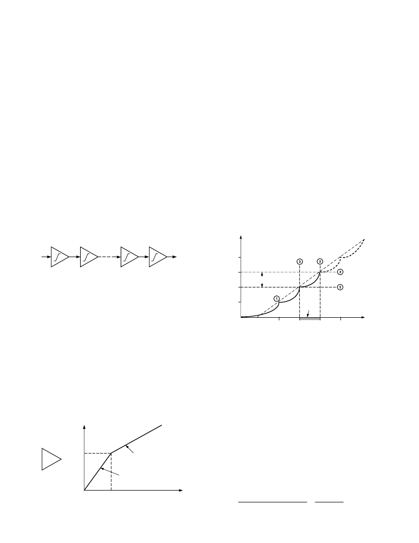
Progressive Compression
Most high speed high dynamic range log amps use a cascade of
nonlinear amplifier cells (Figure 20) to generate the logarithmic
function from a series of contiguous segments, a type of piece-
wise-linear technique. T his basic topology immediately opens
up the possibility of enormous gain-bandwidth products. For
example, the AD8307 employs six cells in its main signal path,
each having a small-signal gain of 14.3 dB (
×
5.2) and a –3 dB
bandwidth of about 900 MHz; the overall gain is about 20,000
(86 dB) and the overall bandwidth of the chain is some 500MHz,
resulting in the incredible gain-bandwidth product (GBW) of
10,000 GHz, about a million times that of a typical op amp.
T his very high GBW is an essential prerequisite to accurate
operation under small-signal conditions and at high frequencies.
Equation 2 reminds us, however, that the incremental gain will
decrease rapidly as V
IN
increases. T he AD8307 continues to
exhibit an essentially logarithmic response down to inputs as
small as 50
μ
V at 500 MHz.
A
V
X
STAGE 1
STAGE 2
STAGE N –1
STAGE N
V
W
A
A
A
Figure 20. Cascade of Nonlinear Gain Cells
T o develop the theory, we will first consider a slightly different
scheme to that employed in the AD8307, but which is simpler
to explain and mathematically more straightforward to analyze.
T his approach is based on a nonlinear amplifier unit, which we
may call an A/1 cell, having the transfer characteristic shown in
Figure 21. T he local small-signal gain
V
OUT
/
V
IN
is A, main-
tained for all inputs up to the knee voltage E
K
, above which the
incremental gain drops to unity. T he function is symmetrical: the
same drop in gain occurs for instantaneous values of V
IN
less
than –E
K
. T he large-signal gain has a value of A for inputs in the
range –E
K
≤
V
IN
≤
+E
K
, but falls asymptotically toward unity for
very large inputs. In logarithmic amplifiers based on this ampli-
fier function, both the slope voltage and the intercept voltage
must be traceable to the one reference voltage, E
K
. T herefore, in
this fundamental analysis, the calibration accuracy of the log amp
is dependent solely on this voltage. In practice, it is possible to
separate the basic references used to determine V
Y
and V
X
and
SLOPE = A
SLOPE = 1
OAE
K
0
E
K
INPUT
A/1
Figure 21. The A/1 Amplifier Function
in the case of the AD8307, V
Y
is traceable to an on-chip band-
gap reference, while V
X
is derived from the thermal voltage kT /q
and later temperature-corrected.
Let the input of an N-cell cascade be V
IN
, and the final output
V
OUT
. For small signals, the overall gain is simply A
N
. A six-
stage system in which A = 5 (14 dB) has an overall gain of
15,625 (84 dB). T he importance of a very high small-signal gain
in implementing the logarithmic function has been noted; how-
ever, this parameter is of only incidental interest in the design of
log amps.
From here onward, rather than considering gain, we will analyze
the overall nonlinear behavior of the cascade in response to a
simple dc input, corresponding to the V
IN
of Equation 1. For
very small inputs, the output from the first cell is V
1
= AV
IN
;
from the second, V
2
= A
2
V
IN
, and so on, up to V
N
= A
N
V
IN
. At
a certain value of V
IN
, the input to the Nth cell, V
N–1
, is exactly
equal to the knee voltage E
K
. T hus, V
OUT
= AE
K
and since there
are N–1 cells of gain A ahead of this node, we can calculate that
V
IN
= E
K
/A
N–1
. T his unique situation corresponds to the lin-log
transition, labeled on Figure 22. Below this input, the cascade
of gain cells is acting as a simple linear amplifier, while for higher
values of V
IN
, it enters into a series of segments which lie on a
logarithmic approximation (dotted line).
V
OUT
LOG V
IN
0
RATIO
OF A
E
K
/A
N–1
E
K
/A
N–2
E
K
/A
N–3
E
K
/A
N–4
(A-1) E
K
(4A-3) E
K
(3A-2) E
K
(2A-1) E
K
AE
K
Figure 22. The First Three Transitions
Continuing this analysis, we find that the next transition occurs
when the input to the (N–1) stage just reaches E
K
; that is, when
V
IN
= E
K
/A
N–2
. T he output of this stage is then exactly AE
K
,
and it is easily demonstrated (from the function shown in Figure
21) that the output of the final stage is (2A–1) E
K
(labeled
on
Figure 22). T hus, the output has changed by an amount (A–1)E
K
for a change in V
IN
from E
K
/A
N–1
to E
K
/A
N–2
, that is, a ratio
change of A. At the next critical point, labeled
, we find the
input is again A times larger and V
OUT
has increased to (3A–2)E
K
,
that is, by another linear increment of (A–1)E
K
. Further analysis
shows that right up to the point where the input to the first cell
is above the knee voltage, V
OUT
changes by (A–1)E
K
for a ratio
change of A in V
IN
. T his can be expressed as a certain fraction
of a decade, which is simply
log
10
(A). For example, when A = 5
a transition in the piecewise linear output function occurs at
regular intervals of 0.7 decade (that is,
log
10
(A), or 14 dB divided
by 20 dB). T his insight allows us to immediately write the Volts
per Decade scaling parameter, which is also the Scaling Voltage
V
Y
, when using base-10 logarithms, as:
V
Y
=
Linear Change inV
OUT
DecadesChange inV
IN
=
A
1
log
10
A
( )
(
)
E
K
(4)
相關(guān)PDF資料 |
PDF描述 |
|---|---|
| AD8309ARU-REEL | 5 MHz.500 MHz 100 dB Demodulating Logarithmic Amplifier with Limiter Output |
| AD8309-EVAL | 5 MHz.500 MHz 100 dB Demodulating Logarithmic Amplifier with Limiter Output |
| AD8309ARU | 5 MHz.500 MHz 100 dB Demodulating Logarithmic Amplifier with Limiter Output |
| AD8309ARU-REEL7 | 5 MHz.500 MHz 100 dB Demodulating Logarithmic Amplifier with Limiter Output |
| AD830 | High Speed, Video Difference Amplifier(高速,視頻差分運(yùn)放) |
相關(guān)代理商/技術(shù)參數(shù) |
參數(shù)描述 |
|---|---|
| AD8307_06 | 制造商:AD 制造商全稱(chēng):Analog Devices 功能描述:Low Cost DC-500 MHz, 92 dB Logarithmic Amplifier |
| AD8307AN | 功能描述:IC LOGARITHMIC AMP 8-DIP RoHS:否 類(lèi)別:集成電路 (IC) >> 線性 - 放大器 - 專(zhuān)用 系列:- 產(chǎn)品培訓(xùn)模塊:Lead (SnPb) Finish for COTS Obsolescence Mitigation Program 標(biāo)準(zhǔn)包裝:60 系列:- 類(lèi)型:可變?cè)鲆娣糯笃?應(yīng)用:CATV 安裝類(lèi)型:表面貼裝 封裝/外殼:20-WQFN 裸露焊盤(pán) 供應(yīng)商設(shè)備封裝:20-TQFN-EP(5x5) 包裝:托盤(pán) |
| AD8307ANZ | 功能描述:IC LOGARITHMIC AMP 8-DIP RoHS:是 類(lèi)別:集成電路 (IC) >> 線性 - 放大器 - 專(zhuān)用 系列:- 產(chǎn)品培訓(xùn)模塊:Lead (SnPb) Finish for COTS Obsolescence Mitigation Program 標(biāo)準(zhǔn)包裝:60 系列:- 類(lèi)型:可變?cè)鲆娣糯笃?應(yīng)用:CATV 安裝類(lèi)型:表面貼裝 封裝/外殼:20-WQFN 裸露焊盤(pán) 供應(yīng)商設(shè)備封裝:20-TQFN-EP(5x5) 包裝:托盤(pán) |
| AD8307AR | 功能描述:IC LOGARITHMIC AMP 92DB 8-SOIC RoHS:否 類(lèi)別:集成電路 (IC) >> 線性 - 放大器 - 專(zhuān)用 系列:- 產(chǎn)品培訓(xùn)模塊:Lead (SnPb) Finish for COTS Obsolescence Mitigation Program 標(biāo)準(zhǔn)包裝:60 系列:- 類(lèi)型:可變?cè)鲆娣糯笃?應(yīng)用:CATV 安裝類(lèi)型:表面貼裝 封裝/外殼:20-WQFN 裸露焊盤(pán) 供應(yīng)商設(shè)備封裝:20-TQFN-EP(5x5) 包裝:托盤(pán) |
| AD8307AR-REEL | 功能描述:IC LOGARITHMIC AMP 8-SOIC T/R RoHS:否 類(lèi)別:集成電路 (IC) >> 線性 - 放大器 - 專(zhuān)用 系列:- 產(chǎn)品培訓(xùn)模塊:Lead (SnPb) Finish for COTS Obsolescence Mitigation Program 標(biāo)準(zhǔn)包裝:60 系列:- 類(lèi)型:可變?cè)鲆娣糯笃?應(yīng)用:CATV 安裝類(lèi)型:表面貼裝 封裝/外殼:20-WQFN 裸露焊盤(pán) 供應(yīng)商設(shè)備封裝:20-TQFN-EP(5x5) 包裝:托盤(pán) |
發(fā)布緊急采購(gòu),3分鐘左右您將得到回復(fù)。