- 您現在的位置:買賣IC網 > PDF目錄373942 > AD8309-EVAL (Analog Devices, Inc.) 5 MHz.500 MHz 100 dB Demodulating Logarithmic Amplifier with Limiter Output PDF資料下載
參數資料
| 型號: | AD8309-EVAL |
| 廠商: | Analog Devices, Inc. |
| 元件分類: | 運動控制電子 |
| 英文描述: | 5 MHz.500 MHz 100 dB Demodulating Logarithmic Amplifier with Limiter Output |
| 中文描述: | 5 MHz.500兆赫和100分貝解調對數放大器輸出限幅 |
| 文件頁數: | 9/20頁 |
| 文件大小: | 311K |
| 代理商: | AD8309-EVAL |
REV. B
AD8309
–9–
labeled
x
on Figure 22. Below this input, the cascade of gain
cells is acting as a simple linear amplifier, while for higher values
of V
IN
, it enters into a series of segments which lie on a logarith-
mic approximation.
Continuing this analysis, we find that the next transition occurs
when the input to the (N–1)th stage just reaches E
K
, that is,
when V
IN
= E
K
/A
N–2
. The output of this stage is then exactly
AE
K
. It is easily demonstrated (from the function shown in
Figure 21) that the output of the final stage is (2A–1)E
K
(la-
beled
≠
on Figure 22). Thus, the output has changed by an
amount (A–1)E
K
for a change in V
IN
from E
K
/A
N–1
to E
K
/A
N–2
,
that is, a
ratio
change of A.
V
OUT
LOG V
IN
0
RATIO
OF A
E
K
/A
N–1
E
K
/A
N–2
E
K
/A
N–3
E
K
/A
N–4
(A-1) E
K
(4A-3) E
K
(3A-2) E
K
(2A-1) E
K
AE
K
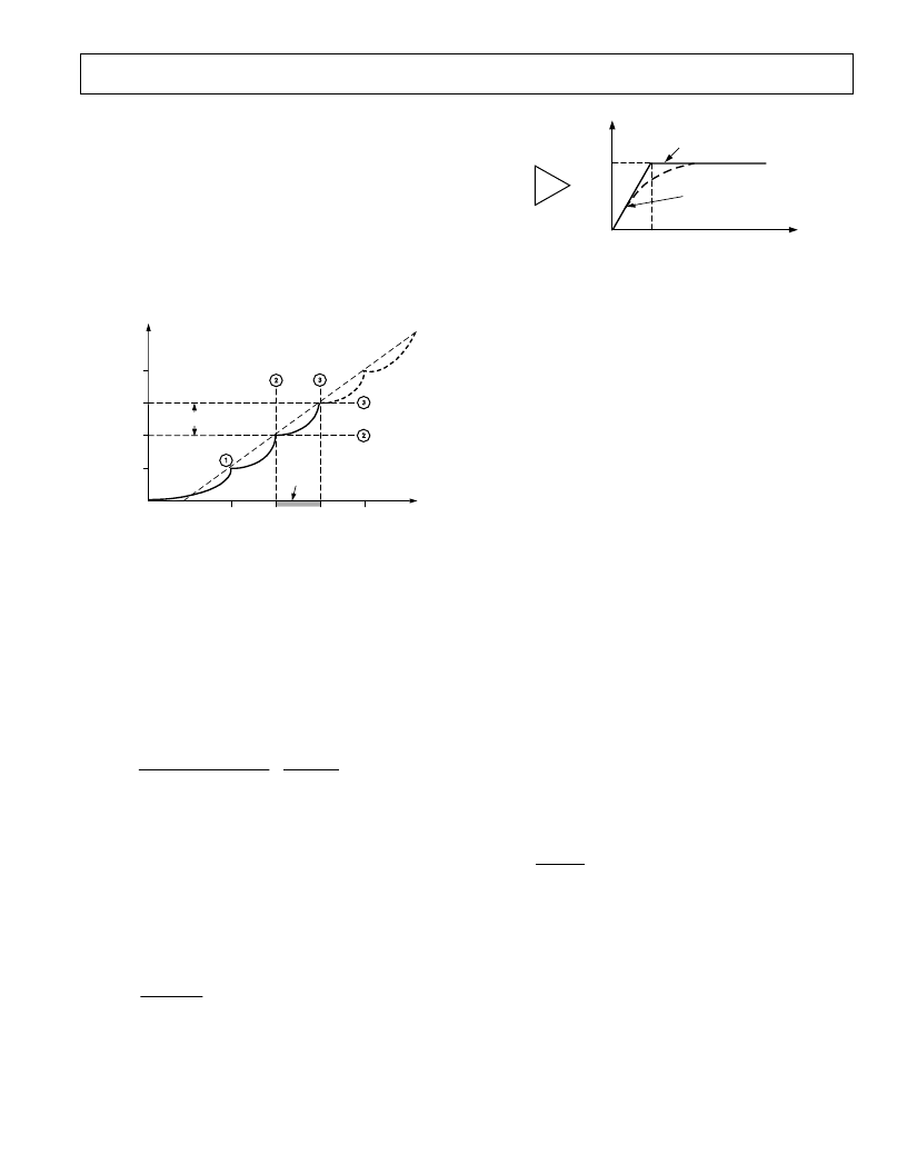
Figure 22. The First Three Transitions
At the next critical point, labeled
z
, the input is A times larger
and V
OUT
has increased to (3A–2)E
K
, that is, by another
linear
increment of (A–1)E
K
. Further analysis shows that, right up to
the point where the input to the first cell reaches the knee volt-
age, V
OUT
changes by (A–1)E
K
for a
ratio
change of A in V
IN
.
Expressed as a certain fraction of a decade, this is simply log
10
(A).
For example, when A = 5 a transition in the piecewise linear
output function occurs at regular intervals of 0.7 decade (log
10
(A),
or 14 dB divided by 20 dB). This insight allows us to immedi-
ately state the “Volts per Decade” scaling parameter, which is
also the “Scaling Voltage” V
Y
when using base-10 logarithms:
V
Linear ChangeinV
DecadesChangeinV
A
log ( )
E
A
Y
OUT
IN
K
=
=
(
– )
1
(4)
Note that only two design parameters are involved in determin-
ing
V
Y
, namely, the cell gain A and the knee voltage
E
K
, while
N, the number of stages, is unimportant in setting the slope of
the overall function. For A = 5 and E
K
= 100 mV, the slope
would be a rather awkward 572.3 mV per decade (28.6 mV/dB).
A well designed practical log amp will provide more rational
scaling parameters.
The intercept voltage can be determined by solving Equation
(4) for any two pairs of transition points on the output function
(see Figure 22). The result is:
V
E
+
A
X
K
/[
– ])
1
N
A
=
(
1
(5)
For the example under consideration, using N = 6,
V
X
evaluates
to 4.28
μ
V, which thus far in this analysis is still a simple dc
voltage.
A/0
SLOPE = 0
SLOPE = A
E
K
AE
K
0
O
INPUT
Figure 23. A/0 Amplifier Functions (Ideal and tanh)
Care is needed in the interpretation of this parameter. It was
earlier defined as the input voltage at which the output passes
through zero (see Figure 19). Clearly, in the absence of noise
and offsets, the output of the amplifier chain shown in Figure 20
can only be zero when V
IN
= 0. This anomaly is due to the finite
gain of the cascaded amplifier, which results in a failure to main-
tain the logarithmic approximation below the “lin-log transition”
(Point
x
in Figure 22). Closer analysis shows that the voltage
given by Equation (5) represents the
extrapolated
, rather than
actual, intercept.
Demodulating Log Amps
Log amps based on a cascade of A/1 cells are useful in baseband
(pulse) applications, because they do not demodulate their input
signal. Demodulating (detecting) log-limiting amplifiers such as
the AD8309 use a different type of amplifier stage, which we
will call an A/0 cell. Its function differs from that of the A/1 cell
in that the gain above the knee voltage E
K
falls to
zero
, as shown
by the solid line in Figure 23. This is also known as the
limiter
function, and a chain of N such cells is often used alone to
generate a hard limited output, in recovering the signal in FM
and PM modes.
The AD640, AD606, AD608, AD8307, AD8309, AD8313 and
other Analog Devices communications products incorporating a
logarithmic IF amplifier all use this technique. It will be appar-
ent that the output of the last stage cannot now provide a loga-
rithmic output, since this remains unchanged for all inputs
above the limiting threshold, which occurs at V
IN
= E
K
/A
N–1
.
Instead, the logarithmic output is generated by
summing the
outputs of all the stages
. The full analysis for this type of log amp
is only slightly more complicated than that of the previous case.
It can be shown that, for practical purpose, the intercept voltage
V
X
is identical to that given in Equation (5), while the slope
voltage is:
V
AE
A
Y
K
=
log ( )
(6)
An A/0 cell can be very simple. In the AD8309 it is based on a
bipolar-transistor differential pair, having resistive loads R
L
and
an emitter current source I
E
. This amplifier limiter cell exhibits
an equivalent knee-voltage of E
K
= 2kT/q and a small-signal
gain of A = I
E
R
L
/E
K
. The large signal transfer function is the
hyperbolic tangent (see dotted line in Figure 23). This function
is very precise, and the deviation from an ideal A/0 form is not
detrimental. In fact, the “rounded shoulders” of the
tanh
func-
tion beneficially result in a lower ripple in the logarithmic con-
formance than that which would be obtained using an ideal A/0
function. A practical amplifier chain built of these cells is differ-
ential in structure from input to final output, and has a low
相關PDF資料 |
PDF描述 |
|---|---|
| AD8309ARU | 5 MHz.500 MHz 100 dB Demodulating Logarithmic Amplifier with Limiter Output |
| AD8309ARU-REEL7 | 5 MHz.500 MHz 100 dB Demodulating Logarithmic Amplifier with Limiter Output |
| AD830 | High Speed, Video Difference Amplifier(高速,視頻差分運放) |
| AD8313ARM-REEL7 | 0.1 GHz-2.5 GHz, 70 dB Logarithmic Detector/Controller |
| AD8313ARM | 0.1 GHz-2.5 GHz, 70 dB Logarithmic Detector/Controller |
相關代理商/技術參數 |
參數描述 |
|---|---|
| AD8309-EVALZ | 制造商:Analog Devices 功能描述:EVAL KIT FOR 5 MHZ-500 MHZ 100DB DEMODULATING LOGARITHMIC AM - Bulk 制造商:Analog Devices 功能描述:EVAL BOARD, AD8309 LOGARITHMIC AMPLIFIER, Silicon Manufacturer:Analog Devices, Silicon Core Number:AD8309, Kit Application Type:RF / IF, Kit Contents:Eval Board AD8309, Features:(Not Applicable) |
| AD830AN | 制造商:Analog Devices 功能描述:Video Amp Single 85MHz 制造商:Analog Devices 功能描述:IC AMP DIFF VIDEO DIP8 830 |
| AD830ANZ | 功能描述:IC VIDEO DIFF AMP HS 8-DIP RoHS:是 類別:集成電路 (IC) >> 線性 - 放大器 - 視頻放大器和頻緩沖器 系列:- 標準包裝:1,000 系列:- 應用:驅動器 輸出類型:差分 電路數:3 -3db帶寬:350MHz 轉換速率:1000 V/µs 電流 - 電源:14.5mA 電流 - 輸出 / 通道:60mA 電壓 - 電源,單路/雙路(±):5 V ~ 12 V,±2.5 V ~ 6 V 安裝類型:表面貼裝 封裝/外殼:20-VFQFN 裸露焊盤 供應商設備封裝:20-QFN 裸露焊盤(4x4) 包裝:帶卷 (TR) |
| AD830AR | 功能描述:IC VIDEO DIFF AMP HS 8-SOIC RoHS:否 類別:集成電路 (IC) >> 線性 - 放大器 - 視頻放大器和頻緩沖器 系列:- 標準包裝:1,000 系列:- 應用:驅動器 輸出類型:差分 電路數:3 -3db帶寬:350MHz 轉換速率:1000 V/µs 電流 - 電源:14.5mA 電流 - 輸出 / 通道:60mA 電壓 - 電源,單路/雙路(±):5 V ~ 12 V,±2.5 V ~ 6 V 安裝類型:表面貼裝 封裝/外殼:20-VFQFN 裸露焊盤 供應商設備封裝:20-QFN 裸露焊盤(4x4) 包裝:帶卷 (TR) |
| AD830AR-REEL | 制造商:Analog Devices 功能描述:Video Amp Single 85MHz |
發布緊急采購,3分鐘左右您將得到回復。